Antibodies 101: Introduction to Gating in Flow Cytometry

When using flow cytometry to analyze your samples, it is necessary to set up a sequence of gates to be able to select and precisely measure your cells of interest. In many experiments you’ll be working with a heterogeneous cell population, for example from a processed piece of tissue, where cells are present that vary in cell type, size, and marker proteins. But even if you are analyzing a homogenous cell population in culture, it is normal to observe diversity in cell size, marker expression, and viability. Gates are the parameters the machine uses to differentiate between variations in those factors.

To understand the principles of gating, you’ll first need to learn a little bit of theoretical background on the different parameters that your gating strategy will be based upon. We’ll try to keep it short though, promise!

FSC and SSC: scattering

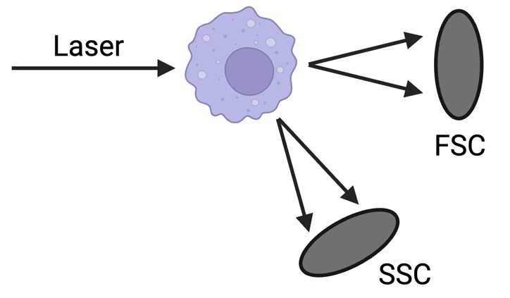
To digitally extract your cells based on their size, the cytometer provides you with two measurements: forward scatter (FSC) and side scatter (SSC). To acquire these measurements, the cytometer illuminates the passing cell with a laser and detects the light scattered by that cell at a low angle (FSC) or large angle (SSC) (Figure 1). FSC values depend on the cell's size, while SSC values depend on the structural complexity inside the cell or on its surface. Bear in mind, the voltage setting of the laser impacts the magnitude of FSC, SSC, and all fluorescent stains. The cytometer's software will allow you to adjust this setting as needed. To figure out the appropriate voltages to observe your cells on a flow plot, you might have to do some testing or ask experienced colleagues.

Figure 1: The laser pulse illuminates the cell and is scattered forward at a low angle (FSC) or to the side at a large angle (SSC). FSC and SSC depend on the cell’s size, morphology, and structural complexity.

Height, Width, and Area

Within FSC and SSC, there are three parameters that are being measured: height (H), area (A), and width (W). The different measures are represented as FSC-A/SSC-A, FSC-H/SSC-H, or FSC-W/SSC-W, respectively. H, A, and W describe the shape of a histogram, which graphically represents the time and intensity of the cell’s illumination (see Figure 2). H describes the maximum signal strength, while W results from the time that the cell spent passing through the laser beam. A is simply the area under the resulting curve. By default, a sample on the flow cytometer (before you set the first gate) will be represented through FSC-A vs. SSC-A, so most people use that setting.

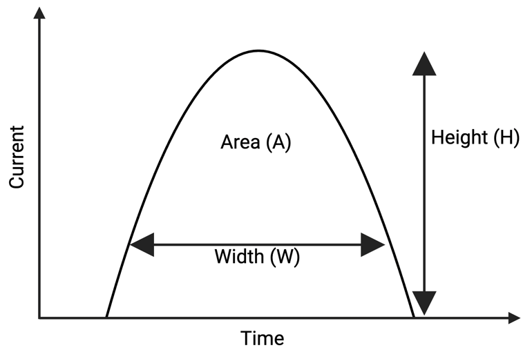Figure 2: As the cell passes through the laser beam and causes it to scatter (FSC/SSC), the detected photons can be represented through a graph of photocurrent vs. time. The resulting histograms is described through maximum current (H), the time the cell needed to pass through the laser (W) and the area under the curve (A).

While flow cytometry can be used for virtually all kinds of experiments and research fields, for any experiment, your first three gates will likely be: the FSC/SSC gate to identify cells, the single cell gate to exclude duplicate events, and the Live/Dead gate to focus your analysis on what’s biologically active. After that, the next gates fully depend on your individual experiment.

Practical example: lymphocytes in a mouse tumor sample

You made it! So much about the theoretical background. Let’s dive into the praxis of gating strategies. As an example, we’ll use one of my previous experiments where I harvested a melanoma tumor from a C57BL/6 mouse and analyzed the tumor-infiltrating lymphocytes of that tumor.

In Figure 3 you can see how I gated out my lymphocyte population from a tumor sample. Many cell types can be found in the tumor microenvironment (tumor cells, immune cells, blood cells and more), each coming with a different size and structural complexity. After several steps of tissue processing prior to running my flow analysis, I can however clearly identify my lymphocyte population (10.7% of all recorded events) based on their expected size. The strong signals close to the graph’s origin mainly stem from cell debris and other small fragments.

Where exactly a given cell population will show up on an FSC/SSC plot, largely depends on cell type and laser voltage. The voltage describes an electric potential that can be applied to the photomultiplier inside the cytometer to increase the electric current and thereby the signal strength. So, we need to adjust the voltage in the cytometer’s software in order to generate signals in a reasonable range. If colleagues in your group already have experience with using flow cytometry, or if you have access to a professional flow core facility, it’s always good to ask around for advice before running your analysis. In this case, I and other lab members had worked with lymphocytes before, so I knew where to look for them on the FSC-A/SSC-A plot.

Figure 3: (A) With the acquisition voltage (not shown) used in my flow analysis I can spot my lymphocyte population distinct from cellular debris and other larger cells. Note, we don’t mind the warning message at the top, as our cells of interest do not lie beyond the dimensions displayed in the plot. (B) A more restrictive gate results in fewer cells being considered for the analysis. (C) A more liberal gate allows more cells to be considered for the analysis. Depending on the following gates, cells that are not of interest can still be gated out later.

Based on personal preference, some people like to make stricter gates while some like to make looser ones (Figure 3). A more “liberal” gate in the beginning should not have a great impact on your analysis, and I often choose a looser gate here. I am not worried about including irrelevant events in my analysis, as these will get excluded through further, more specific gates (single cells, live cells, my marker stains of interest). Let’s double-click inside our gate and proceed to the next plot!

Pro tip! If you only get very few events at the end of your gating pipeline, it might be worth going back and loosening the FSC/SSC gate.

Single-cell gating

Once you have identified and gated on your cells of interest, you will likely need to exclude all duplicate events (two cells stuck together) from your single cells, as duplicates can’t be reliably analyzed on their staining signals. For this, you’ll need to gate based on the proportion between H and A (or W and A) within the same type of scatter. Here I employed an FSC-H / FSC-A gate, but an SSC-H / SSC-A gate would work just as fine (Figure 4). As H and A scale in proportion (while H and W do not; see Figure 2), single cell events will show up in a straight line one the plot, while duplicates deviate from that pattern.

A.                                                                                                         B. 

Figure 4: (A) Using the proportional relationship between FSC-H and FSC-A we can gate on single cells and exclude any events where multiple cells were clumped together. (B) Instead of FSC, one is free to use SSC for a single cell gate. However, make sure to compare H and A (or W and A).

Live/Dead Gating

Having gated my single lymphocyte cells, I now want to exclude all dead cells from my analysis. For this measurement, I used a fluorescent dye that can only enter dead cells, while living cells can protect themselves from it. So here, I actually want to gate on my negative, unstained population, which I can clearly differentiate from the positive one (Figure 8). Note that in many cases a stain will not result in clearly distinct positive and negative populations. Oftentimes, you’ll be presented with a trend of two populations with basically a smear in between. Again, it can depend on the type of stain whether a tighter or looser gate makes sense. Here, luckily, the vast majority of my cells of interest lies within a clear negative population.

When you’re interested in measuring a population based on a fluorescent stain, you might be wondering which second measurement to choose for graphically displaying your events. You are free to choose any size-related parameter, such as FSC-H, FSC-A, SSC-H, SSC-A, etc. You’ll notice that while the height of your events changes, the separation pattern of positive vs. negative signal remains the same (Figure 5).

A.                                                                                                        B. 

Figure 5: (A) A gate to select the negative live population from my live-dead staining. (B) Changing the y-axis from SSC to FSC can alter the positioning and shape of the populations displayed. As the separation pattern largely stays the same and does not impact my ability to draw a proper gate, I am free to choose either one to use.

With our first three gates out of the way, it’s time to move on to my experimentally-specific gates.

Two-dimensional staining (quadrant gating)

For our last example plot, I will show you a combination of two stains, in this case through conjugated antibodies targeting the cell surface markers CD11 (anti-mouse CD11b-BV510), which is present on dendritic cells but not T cells, and CD8 (anti-mouse CD8b-PerCP-Cy5.5), which is present on cytotoxic T killer cells but not dendritic cells.

Using a graph displaying both stains, I can quickly separate T killer cells (CD8⁺) from dendritic cells (CD11b⁺) using a quadrant gate. Within my “lymphocyte + single cell + live” population, acquired from the previous gating pipeline, about 53% of my cells are dendritic cells and ~13% are CD8⁺ T cells. Around 34% of the cells are neither of the two cell types (likely B cells and others). Almost no cells stain positively for both markers. When comparing two markers simultaneously, we commonly describe the resulting populations as double positive (DP, Q2), single positive (SP, Q1/Q3) or double negative (DN, Q1). If I wish to employ a more refined gating strategy, I can, of course, also draw multiple individual gates around the populations of interest (Figure 6).

A.                                                                                               B. 

 

Figure 6: (A) A flow plot showing two stains in relation to each other. Using a quadrant gate, I can divide my cell population into DN, DP and SP (for each stain respectively). (B) Instead of a quadrant gate, I am free to use multiple individual gates. Note that in this case, square gates were used. 

Congratulations! You’ve just learned the basic principles of gating in flow cytometry. Let’s briefly recapitulate what we’ve covered in this blog post. First, you learned about the types of scattering that occur when a cell is pulsed by the laser. Within each type of scattering, you also discovered that there are three parameters — H, W, and A — describing the intensity and duration of the detected signal. Using a practical example of lymphocytes from a mouse tumor, you’ve learned how to read an FSC/SSC plot and how to use H vs. A to distinguish single cells from duplicates. Lastly, you learned which gates should always be included in your analysis, regardless of your experiment, and how you can combine two colors (stains) to visualize four populations at once.

 

Paul Heisig is a Research Associate in the lab of Arlene Sharpe at Harvard Medical School. His projects include investigating negative regulators of T cells and cytokine signaling in tumor immunity. When he's not in the lab, Paul enjoys weight lifting, sailing, and reading.

 

---

More resources on the Addgene blog

Antibodies 101: Flow Cytometry 

Antibodies 101: Reading a Flow Plot

Antibodies 101: Conventional vs. Spectral Flow Cytometry