Welcome to our deep dive series, which aims to increase your understanding and technical proficiency with common applications - now let’s dive right in!
You know qPCR is most commonly used to measure relative quantification of mRNA, which can be used as a proxy measure for differences in protein expression. (If you're just getting started, check out our Introduction to PCR.) But if you're ready to go beyond the 101 and take your understanding to the next level, read on for more in-depth tips on probe chemistries, primer optimization, controls, and analysis.
As a rule of thumb, you can assume that qPCR can accurately detect expression differences of twofold or greater with good statistical significance (Taylor, 2017). With the right conditions and parameters, some people find it can detect even smaller differences, and it can even be used to detect a single copy of a transcript. But this sensitivity can sometimes cause as many issues as it solves, so understanding and using the application correctly is imperative.
Picking your chemistry
The two most common qPCR chemistries are hydrolysis probes (which you probably know as TaqMan) and dsDNA dyes (commercial name: Sybr). However, there are other chemistries available and they can be the more optimal choices at times. For example, chemistries that rely on hairpin design of probes/primers often offer higher allelic specificity, due to the need for the target:probe/primer bonds to be more stable than the hairpin bond.
Alternatively, chemistries that combine the primer and probe into a single molecule often work better for rapid-cycle PCR, such as the LightCycler, as it reduces the primer/probe actions to a single step. Scorpion chemistry in particular has been reported to work well in the Lightcycler while being relatively easy to multiplex (Thellwell, 2000). See Table 1 for a comparison of features of several commonly used chemistries)
|
Chemistry |
Background noise |
Probe |
Allelic specificity |
Can be multiplexed |
Single amplicon validation technique |
|
Hydrolysis Probes (Taqman) |
Low; can be reduced with a double-quencher design |
Yes, one |
Yes |
Yes |
Agarose gel or uMelt analysis |
|
dsDNA dye (Sybr) |
High |
No |
No |
No |
Melt curve |
|
Hybridization Probes |
Low |
Yes, two |
Yes |
Yes |
Agarose gel or uMelt analysis |
|
Hairpin probes |
Low |
Yes, one |
Yes |
Yes |
Agarose gels |
|
Scorpions |
Low |
Probe is on a hairpin structure included in the 5’ primer |
Yes |
Yes. |
Agarose gel |
|
LUX fluorogenic primers |
Low |
Single self-quenching fluorescent molecule connected to a primer |
No |
Yes |
Agarose gel |
|
Sunrise primers
|
Low |
Reporter and quencher on hairpin structure included in primer |
Yes |
Yes |
Agarose gel |
| Table 1: Features of various qPCR chemistries. Adapted from Wong, 2018 |
Primers
Design of primers and probes
Primer design, of course, could easily be its own deep dive, but here are some general helpful principles (and I recommend Bustin, 2017 for a more in-depth review.)
- Your amplicon should be between 70-200 bp long
- With ΔΔCT analysis you’ll want to stay under 150 bp long
- Annealing temperature should be 60-65°C
- For qPCR, the important primer variable is the annealing temperature, not the melting temperature. Though you’ll want to predict this value using BLAST, you’ll need to experimentally verify once you’ve received the primers.
- Melting temperature should be ~60°C (between 50 and 65, with no more than 3 degrees between the two Tms)
- Aim for 50-60% GC content, preferably weighted towards the ends of the primers.
- Concentration of primers should be between 100 and 400 nm and must be optimized experimentally.
- Probe should have a melting temperature 5-10 degrees above the primer and be at least 25 bp away from each primer, ideally located close to either the forward or the reverse primer.
There is a list of useful primer design resources in the References and Resource section.
Validation
Once designed, your primer and probe set needs to be validated and your reaction optimized. You’ll want to run gradients for optimal annealing temperature and optimal primer concentration; check for primer dimers; and validate assay efficacy with a standard curve. If relying on previously-generated validation data, be aware that different machines, samples, and treatments may affect the assay. It’s unusual to need to adjust amounts of reagents in your chemistry, unless running a multiplex reaction or on a rapid cycle machine.
Melt Curves
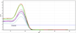
An advantage of Sybr chemistry is the ability to run a melt curve to validate your primers. This separate thermocycle allows you to measure the intensity of signal over an entire cycle. Since signals are produced by the presence of double-stranded DNA, when temperatures are high, signal intensity should be low, reflecting the presence of primarily denatured (single-stranded) DNA. As the temperature drops, single intensity should smoothly increase as the DNA amplicon transitions from single-stranded to double-stranded, and finally, drop once more during a final temperature increase. If there is a single amplicon, there should only be one peak, as everything should be denaturing or annealing at the same temperatures. If there are multiple amplicons, or primer dimers forming, the curve will show multiple peaks.
|
(a)
|
| Fig. 1: Melt curves showsing (a) a single peak, indicating one amplicon and no primer dimers. (b) A shoulder peak indicating primer dimers. (c) A double peak indicating 2 amplicons. Image credits (respectively): Zuzanna K. Filutowska; Selma, 2019; Trampuz, 2003. |
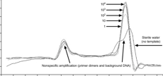 (c)
(c) 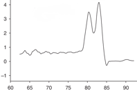
You’ll note this melt curve does rely on the assumption that there is a smooth, single-step transition between ssDNA and dsDNA. This is not true for all amplicons; if your amplicon is AT-rich or has a secondary structure, you may see a double peak even with a single product. In that case, you’ll want to validate your primer/probe through another means, such as an agarose gel or uMelt analysis (Downey, 2014).
Agarose gels
A quick way to validate your primer probe is by running your qPCR product on an agarose gel, then cutting out and sequencing the band for verification. Primer dimers will often show up as a smear or band around 30-50 bp.
uMelt analysis
uMelt is an online tool that uses the amplicon sequence and thermodynamic and experimental parameters (neighbor stacking energies, loop entropy effects, cation concentrations and a temperature range) to predict PCR melting curves and dynamic melting profiles (Dwight, 2011).
Reference Genes
Choosing a set of reference genes deserves more attention than it usually receives. Different reference genes have shown to have as much as sixfold variation in expression levels reported (Biassoni, 2014), so you’ll want to ensure that your reference genes are suitable for your cell lines and/or tissue types.
Please do note my oh-so-subtle use of reference genes, plural. Your data will be much improved if you move to using multiple reference genes whenever possible (Vandesompele, 2002), and it's possible to multiplex your reference genes to save on plate space.
For many cell lines and tissue types, appropriate reference genes (and supporting data) are often documented in the literature. However, it is not enough to rely on a reference gene being a common choice - the frequently used GAPDH has noted issues as a reference gene (Higgins, 2000; Ref, Zhu, 2002), though there are cases in which it is an appropriate choice (Panina, 2018). Look for studies specifically aimed at determining the best options for a particular cell or tissue type (such as here, here, or here).
If you’re working with samples that have not been documented in the literature, a geNorm study (Vandesompele, 2002) will help you select the appropriate reference genes - and it is well worth your time to do one (Biassoni, 2014).
At the bench
As a highly sensitive technique, qPCR needs a steady pair of hands to produce reliable and reproducible data. Here are some tips to help you in your execution:
- Accuracy is not as important as precision for relative quantification. A consistent 5% positive error across the plate is fine; a 5% positive error on one side and a 5% negative error on the other will introduce unwanted variation into your data. Try different types of pipettes and pipetting methods to find what’s most consistent in your hands.
- When using multichannels, set up your plate in a way that will tell you if you have pipetting errors on the edges of the plate. Compare the CT values within each set of triplicates to understand variation due to technical error.
- Plate readouts can be affected by plate type or tubes, sealing method, and other small variations in consumables. Track and record these details for reproducibility’s sake!
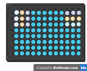 |
| Fig. 2: Setting up triplicates in multiple configurations can help you identify pipetting or evaporation errors. And if time allows, you can fit in a quick game of Connect Four! Image created in BioRender. |
Passive Reference Dyes
Whatever your pipetting method, some variation will occur. A passive reference dye, such as ROX, can help normalize for that. Passive reference dyes are inert fluorescent dyes that are not dependent on amplification of the DNA; they are, however, affected by bubbles in wells, variations in volume, or machine surge errors and allow for well-to-well normalization of signal. They are often included in commercial sets and most machines have a protocol that automatically performs the normalization step.
Machines
Most general-use protocols, unless otherwise specified, were likely developed on the ABI 7000 series. If you’re using a different brand of qPCR machine, especially if you’re using a rapid-cycle machine such as a LightCycler, you’ll likely need to re-optimize protocols for that machine. (Teo, et al, 2002; see paper for more information on optimizing for LightCycler machines.)
Multiplexing
It is possible to multiplex qPCR when using fluorescent probe-based chemistry - theoretically, up to five or six reactions in a single well. In practice, multiplexing is quite difficult and requires significant optimization to ensure the results are correct. Primers and probes can interfere with amplification reactions, and reagents can be used up quickly by abundant transcripts, leading to falsely lowered levels for less abundant transcripts. However, adding too many reagents can prevent your reaction from reaching the plateau stage after exponential amplification, making it difficult to properly analyze your data.
To develop a multiplex reaction, each target in the reaction should be compared to an individually run sample when developing the protocol and optimized until the multiplexed and individual values match across the board. If the samples or sample conditions change, the multiplexed protocol may have to be re-optimized.
While troublesome, multiplexing your reference gene set can save significant plate space and may be worth the initial effort of setting it up for larger or frequently analyzed sample types and sets.
|
🔥Hot Tip🔥 The ABI machines automatically record fluorescent data on all channels - helpful if you forget to set the channel wavelength before you run the plate. |
Analyzing
There are a number of methods available for analyzing qPCR data, most with plug-and-play Excel spreadsheets available for easy analysis. These useful tools don’t excuse you from understanding how the analyses work - you do need to make sure the assumptions in your dataset match the assumptions in your analysis method.
ΔΔCT/CQ method
One of the most commonly used methods is the ΔΔCT/CQ method, which gives an RQ value representing the fold change of each sample compared to your control. But as we said previously, just because it’s used often doesn’t mean it’s right for your experiment! The model assumes the amplification kinetics of the target and control genes are fairly equal, an assumption that is not always verified before use. If you’re using the ΔΔCT method and you’re not sure if your amplification efficiencies match, you’ll need to run a validation assay in which serial dilutions for the target and housekeeping genes are run and the difference in CT values is plotted against the log input concentration for each dilution. For the ΔΔCT method to be accurate, the absolute value of the slope generated should be less than 0.1.
If you suspect that amplification efficacy differences may be a concern in your reaction, analysis techniques that use raw data corrections are a better choice (Tichopa, 2003. Marino, 2003) - an important note, as the other most commonly used method is the Standard Curve method. See Table 2, (adapted from Wong, 2018) for a comparison of different analysis methods.
|
Method |
Standard Curve? |
Amplification Efficacy Calculation |
Amplification Efficacy Assumptions |
|
Standard Curve |
Yes |
Standard Curve |
No experimental sample variation |
|
ΔΔCT |
No |
Standard Curve |
reference=target |
| No |
Standard Curve |
sample=control |
|
| No |
Raw Data |
researcher defines log-linear phase |
|
| No |
Raw Data |
Reference and target genes can have different efficacies |
|
| No |
Raw Data |
Statistically defined log-linear phase |
| Table 2: A comparison of different qPCR analysis methods. Table adapted from Wong, 2018. |
|
🔥Hot Tip🔥 Negative fold changes in ΔΔCT are represented by RQs between 0 and 1. Flipping your experimental and control values during analysis can allow you to see this fold change as a positive difference (RQ>1), which may be easier to conceptualize. Just remember to switch them back before reporting the data! |
Statistical analysis
Getting your RQ value isn’t the end of your analysis process. You’ll still need to do statistical analysis to determine if there are any significant differences between your experimental values and your controls. ANOVA, t-test, multiple regression analysis, and non-parametric analogous Wilcoxon tests have all been shown to give similar results, so you only need to pick your favorite (...er, whichever one uses assumptions that match your data set, that is.) Yuan, 2006 has a good overview of different statistical analysis methods that pair well with slightly modified CT analysis, so pick one and use it! Tempting as it may be to skip this step, remember we here at Addgene frown upon statistical laxness in all its forms.
Reporting your data
Once you’ve done the work to produce excellent and reliable qPCR data, you’ll of course want to share it so others can provide you with the highest form of flattery - imitation! Use the MIQE guidelines (Bustin, 2009) to ensure you’re recording and reporting the right information so others can reproduce your efforts. And if you need to know more, take a look at their 551 page e-book on applying MIQE guidelines! With these kinds of resources, you will soon become a qPCR master.
References and Resources
References
Biassoni R; Raso A. (eds.), Quantitative Real-Time PCR: Methods and Protocols, Methods in Molecular Biology, vol. 1160, DOI 10.1007/978-1-4939-0733-5_3, © Springer Science+Business Media New York 2014
Bustin S; Huggett J. qPCR primer design revisited. Biomolecular Detection and Quantification. Volume 14. 2017, Pages 19-28, ISSN 2214-7535, https://doi.org/10.1016/j.bdq.2017.11.001.
Bustin SA; Benes V; Garson JA; Hellemans J; Huggett J; Kubista M; Mueller R; Nolan T; Pfaffl MW; Shipley GL; Vandesompele J; Wittwer CT. The MIQE guidelines: minimum information for publication of quantitative real-time PCR experiments. Clin Chem. 2009 Apr;55(4):611-22. doi: 10.1373/clinchem.2008.112797. Epub 2009 Feb 26. PMID: 19246619.
Downey N. Interpreting melt curves: An indicator, not a diagnosis. IDT, 2014.
Dwight Z; Palais R.; Wittwer CT. uMELT: prediction of high-resolution melting curves and dynamic melting profiles of PCR products in a rich web application, Bioinformatics, Volume 27, Issue 7, 1 April 2011, Pages 1019–1020, https://doi.org/10.1093/bioinformatics/btr065
Freeman WM; Walker SJ; Vrana KE. 1999. Quantitative RT-PCR: pitfalls and potential. BioTechniques 26:112–115.
Marino JH; Cook P; and Miller KS. 2003. Accurate and statistically verified quantification of relative mRNA abundances using SYBR Green I and real-time RT-PCR. J. Immunol. Methods 283:291–306.
Panina, Y., Germond, A., Masui, S. et al. Validation of Common Housekeeping Genes as Reference for qPCR Gene Expression Analysis During iPS Reprogramming Process. Sci Rep 8, 8716 (2018). https://doi.org/10.1038/s41598-018-26707-8
Suzuki T; Higgins PJ; Crawford DR. Control selection for RNA quantitation. Biotechniques. 2000 Aug;29(2):332-7. doi: 10.2144/00292rv02. PMID: 10948434.
Taylor SC; Laperriere G; Germain H. Droplet Digital PCR versus qPCR for gene expression analysis with low abundant targets: from variable nonsense to publication quality data. Sci Rep 7, 2409 (2017). https://doi.org/10.1038/s41598-017-02217-x
Taylor, SC; Nadeau, K; Abbasi, M; Lachance, C; Nguyen, M; Fenrich, J. The Ultimate qPCR Experiment: Producing Publication Quality, Reproducible Data the First Time, Trends in Biotechnology, Volume 37, Issue 7, 2019, Pages 761-774, SSN 0167-7799, https://doi.org/10.1016/j.tibtech.2018.12.002.
Teo IA; Choi JW; Morlese J; Taylor G; Shaun S. LightCycler qPCR optimisation for low copy number target DNA. Journal of Immunological Methods 270 (2002) 119 – 133
Tichopad A; Dilger M; Schwarz G; Pfaffl MW. 2003. Standardized determination of real-time PCR efficiency from a single reaction set-up. Nucleic Acids Res. 31:e122.
Thelwell N; Millington S; Solinas A; Booth J; Brown T. Mode of action and application of Scorpion primers to mutation detection, Nucleic Acids Research, Volume 28, Issue 19, 1 October 2000, Pages 3752–3761, https://doi.org/10.1093/nar/28.19.3752
Wong M; Medrano J. Real-time PCR for mRNA quantitation. Biotechniques, 1, 30 (2018). https://doi.org/10.2144/05391RV01
Yuan JS; Reed A; Chen F. et al. Statistical analysis of real-time PCR data. BMC Bioinformatics 7, 85 (2006). https://doi.org/10.1186/1471-2105-7-85
Zhu G; Chang Y; Zuo J, Dong X, Zhang M, Hu G, Fang F. Fudenine, a C-terminal truncated rat homologue of mouse prominin, is blood glucose-regulated and can up-regulate the expression of GAPDH. Biochem Biophys Res Commun. 2001 Mar 9;281(4):951-6. doi: 10.1006/bbrc.2001.4439. PMID: 11237753.
Primer design resources
PrimerBlast
DINAmel
Mfold
BLAST
Ensembl
More resources on the Addgene blog
Digital Droplet PCR for AAV Quantification
Plasmid Cloning by PCR


Leave a Comment